mean-field solver

Some background

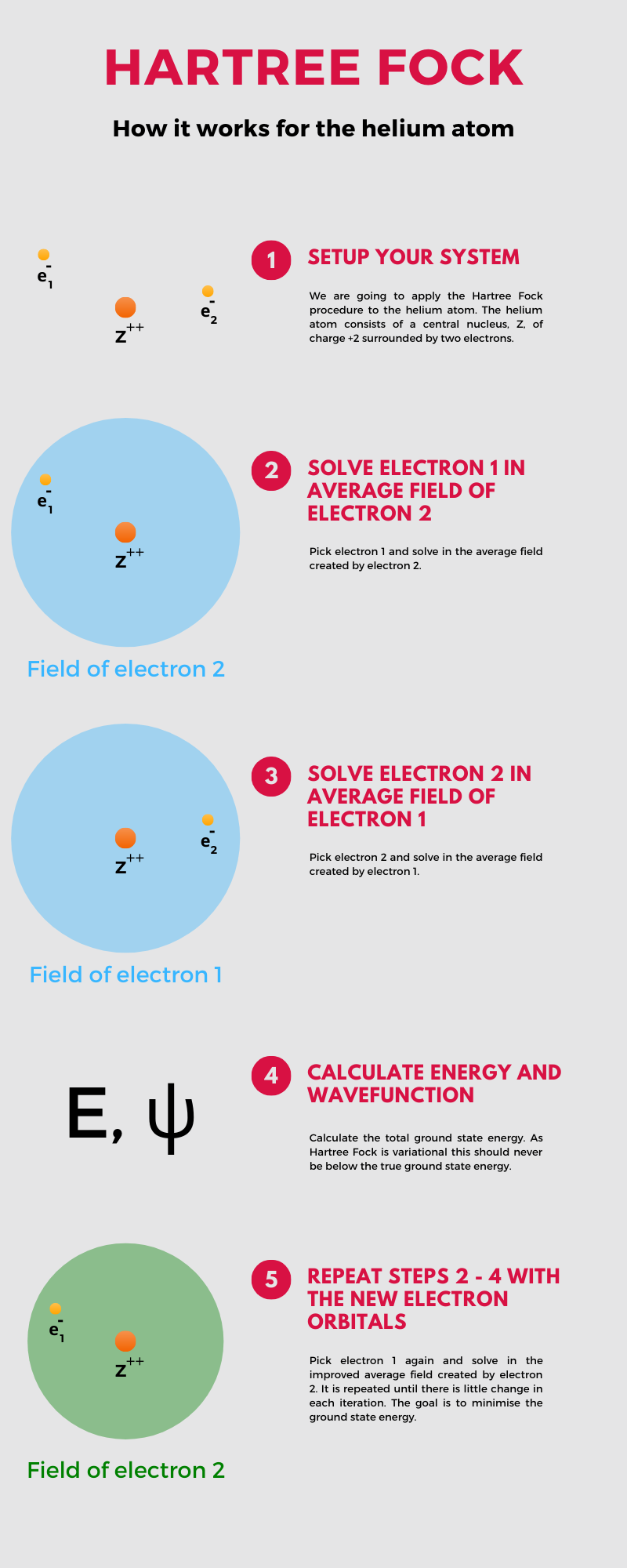
What is a mean field solver and why do we need it?

Solving many-body systems such as a hellium atom in chemistry (reference I used here):

Why is it useful?

• If we tried to solve N particles with M distinct states exactly, the full Hilbert space is M^N. Mean-field maps into a much smaller non-interacting system of size M N
• Quantitative accuracy is either hit or miss, but gives a good understanding of the qualitative behaviour of the system.

General idea through an example

The Ising model

Consider an Ising model:

with the Hamiltonian (straight from wikipedia):

H=-J\sum _{\langle i,j\rangle }s_{i}s_{j}-h\sum _{i}s_{i}

where s_i is the spin of the ith particle, J is the exchange coupling, and h is the external magnetic field. The sum is over nearest neighbours.

Identifying and applying mean field

It is an interacting problem and thus a headache to solve. Rather than consider all the particles, lets consider a single particle in an effective field of other spins. To do that, lets define the average spin m_{i}\equiv \langle s_{i} \rangle and re-write the s_i s_j product into:

s_i s_j = m_i m_j + m_i \delta s_j + m_j \delta s_i + \delta s_i \delta s_j

if we assume the fluctuations are small, then at the very least the last term can be neglected:

s_i s_j \approx m_i m_j + m_i \delta s_j + m_j \delta s_i = m_i s_j + m_j s_i - m_i m_j

and thus the Hamiltonian becomes:

H\approx H^{\text{MF}}\equiv -J m \sum _{\langle i,j\rangle }(2 s_{i} - m)-h\sum _{i}s_{i}

where for simplicity I also assumed that the average spin m_i is constant for all particles.

Self-consistency

The average mean-field m here acts as a variable, or better yet, an initial guess. After solving H_{\text{MF}}, we need to make sure that the m is self-consistent with the new s_i:

m = \frac{1}{N} \sum_i^N \langle s_i \rangle.

So we re-calculate m, plug it back into the equation of H_{\text{MF}}, and repeat until m converges.

Summary

1. Identify the mean-field variables and construct the mean-field Hamiltonian.
2. Guess the initial mean-field.
3. Self-consistency loop:
   1. Solve the mean-field Hamiltonian H_{\text{MF}} for the given mean-field.
   2. Calculate the new mean-field.
   3. Check convergence. If not converged, go back to step 3.1. with the new mean-field.
4. ???
5. Profit.

Why waste time with this?

Interacting systems have become quite hot research field in condensed matter physics (I mean, take a look at graphene). However, numerical packages to solve them on tight-binding systems lack the following:

• Not many well-maintained packages.
• Code is needlessly complex and documentation is lacking.
• Lack generality.

Idea behind our implementation

Identifying mean-fields

Real Space

You can find the whole theory here.

Here the the main points. A general particle number preserving interaction with all mean-fields can be written as a sort of Wick's contraction:

V = \frac{1}{2}\sum_{ijkl} v_{ijkl} c_i^{\dagger} c_j^{\dagger} c_l c_k \approx \frac12 \sum_{ijkl} v_{ijkl} \left[ \langle c_i^{\dagger} c_k \rangle c_j^{\dagger} c_l - \langle c_j^{\dagger} c_k \rangle c_i^{\dagger} c_l - \langle c_i^{\dagger} c_l \rangle c_j^{\dagger} c_k + \langle c_j^{\dagger} c_l \rangle c_i^{\dagger} c_k \right] (we neglect superconductivity)

here i,j,k,l label any degree of freedom written on a tight-binding grid, so we maintain full generality.

The mean-fields are in terms of second quantization operators, but how do we translate the problem to a tight-binding grid/matrix problem?

\langle c_i^{\dagger} c_j\rangle = \langle \Psi_F|c_i^{\dagger} c_j | \Psi_F \rangle

whereas |\Psi_F \rangle = \Pi_{i=0}^{N_F} b_i^\dagger |0\rangle. To make sense of things, we need to transform between c_i basis (position + internal dof basis) into the b_i basis (eigenfunction of a given mean-field Hamiltonian):

c_i^\dagger = \sum_{k} U_{ik} b_k^\dagger

where U is the matrix of eigenvectors of the mean-field Hamiltonian:

U_{ik} = \langle{i|\psi_k} \rangle.

That gives us:

c_i^{\dagger} c_j = \sum_{k, l} U_{ik} U_{lj}^* b_k^\dagger b_{l}

and its expectation value gives us the mean-field ... field F_{ij}:

F_{ij} = \langle c_i^{\dagger} c_j\rangle = \sum_{k, l} U_{ik} U_{lj}^* \langle \Psi_F| b_k^\dagger b_{l}| \Psi_F \rangle = \sum_{k} U_{ik} U_{kj}^{*}

Coming back to the interaction, under mean-field and on our chosen tight-binding grid it reads:

V_{nm} \approx -\sum_{ij} F_{ij} \left(v_{inmj} - v_{injm} \right)

In the simple case of a Coulomb interaction, the potential reads:

V_{nm} = -F_{mn} v_{mn} + \sum_{i} F_{ii} v_{in} \delta_{nm}

where the second term is the Direct Coulomb interaction, and the first term is the exchange interaction.

k-space or translational invariance case

The above works for a finite sized tight-binding model, but what about a periodic system? In that case, we can use the Fourier transform to write the mean-field Hamiltonian in k-space. I'll spare you the details, the final result reads:

V_{nm}(k) =-F_{mn}(k) \circledast v_{mn}(k) + \sum_{p} \rho_{p} v_{pn}(0) \delta_{nm}

where \rho_{p} is the particle density at unit cell site p, averaged over a k-grid:

\rho_{p} = \int F_{pp}(k) dk

Once again, the first term (exchange) is purely responsible for the hopping whereas the second term (direct) is a potential term coming from the mean-field.

Scaling of the algorithm

Lets say M is the number of degrees of freedom within the unit cell, and N is the number of k-points along a direction (we consider 2D problem here). Then the following steps limit the scaling of the algorithm:

• Eigenvalue problem for each k-point: O(N^2 M^3).
• Convolution in k-space: O(N^4 M^2). In this case, this is the most expensive step.